Tutorial
Introduction
nmrglue is a python module for reading, writing, and interacting with the spectral data stored in a number of common NMR data formats. This tutorial provides an overview of some of the features of nmrglue. A basic understanding of python is assumed which can be obtained by reading some of the python documentation. The examples in this tutorial can be run interactively from the python shell but the use of an enhanced python shell which provides non-blocking control of GUI threads, for example ipython, is recommended when trying the examples which use matplotlib. The sample data using in this tutorial is available is you wish to follow along with the same files.
The software can also be used in Google Colabs - see details below.
Reading NMR files
nmrglue can read and write to a number of common NMR file formats. To see
how simple this can be let’s read a 2D NMRPipe file. (Note: If you need an example
dataset, use the one provided here, and replace test.fid or test.ft with the names
of the files ending in .fid or .dat).
>>> import nmrglue as ng
>>> dic,data = ng.pipe.read("test.fid")
Here we have imported the nmrglue module and opened the NMRPipe file
test.fid. nmrglue contains a number of modules for reading and writing NMR
files and all of these modules have a read function which opens a file
or directory containing NMR data, reads in any necessary information, and loads
the spectral data into memory. The read function returns a 2-tuple
containing a python dictionary with file and spectral parameters and a
numpy array object containing the numeric
spectral data. Currently the following file formats are supported by nmrglue
with the associated module:
Module |
File Format |
Reference |
|---|---|---|
bruker |
Bruker |
https://www.bruker.com/service/information-communication/user-manuals/nmr.html |
pipe |
NMRPipe |
|
sparky |
Sparky/Poky |
|
varian |
Varian/Agilent |
|
rnmrtk |
Rowland NMR Toolkit |
|
jcampdx |
JCAMP-DX |
|
nmrml |
NMR Markup Language |
|
simpson |
Simpson |
https://inano.au.dk/about/research-centers-and-projects/nmr/software-and-tools/downloads/ |
spinsolve |
Magritek or JCAMP-DX |
|
tecmag |
Technology for Magnetic Resonance |
Examining the data object in more detail:
>>> data.ndim
2
>>> data.shape
(332, 1500)
>>> data.dtype
dtype('complex64')
We can see that this is a two dimensional data set with 1500 complex points in the direct dimension and 332 points in the indirect dimension. nmrglue takes care of converting the raw data in the file into an array of appropriate type, dimensionality, and quadrature. For complex data the last axis, typically the direct dimension, is converted to a complex data type. The other axes are not converted.
In some cases, not all of the information needed to represent the spectral data as a well formed numpy array is stored in the file, or the values determined automatically are incorrect. In many of these cases, this information can be specified directly in the function call.
For example, the read function in the varian module sometimes cannot
determine the shape or fid ordering of 3D files correctly. These parameters
can be explicitly provided in the function call with the shape and torder
keywords. See nmrglue.varian for details.
Universal dictionaries
In addition to the spectral data, the read function also determines
various spectral parameters that were stored in the file and stores them in a
python dictionary:
>>> dic["FDF2SW"]
50000.0
>>> dic["FDF1LABEL"]
'15N'
Here we see NMRPipe files stores the spectal width of the direct dimension (50000.0 Hz) and the name of the indirect dimension (15N) as well as a number of additional parameters.
Some file formats describe well the spectral data, listing a large number of
parameters, other only a few. In addition, different formats express
parameters in different units and under different names. For users who are
familiar with the specific file format or are working with only a single file
type, this is not a problem; the dictionary allows direct access to these
parameters. If a more uniform listing of spectral parameters is desired, the
guess_udic function can be used to create a ‘universal’ dictionary.
>>> udic = ng.pipe.guess_udic(dic,data)
>>> udic.keys()
['ndim', 0, 1]
>>>
This ‘universal’ dictionary of spectral parameters contains only the most fundamental parameters, the dimensionality of the data, and a dictionary of parameters for each axis numbered according to the data array ordering (the direct dimension is the highest numbered dimension). The axis dictionaries contain the following keys:
Key |
Description |
|---|---|
car |
Carrier frequency in Hz. |
complex |
True for complex data, False for magnitude data. |
encoding |
How the data is encoded, ‘states’, ‘tppi’, etc. |
freq |
True for frequency domain data, False for time domain. |
label |
String describing the axis name. |
obs |
Observation frequency in MHz. |
size |
Dimension size (R|I for last axis, R+I for others) |
sw |
Spectral width in Hz. |
time |
True for time domain data, False got frequency domain. |
For our 2D NMRPipe file, these parameters for the indirect dimension are:
>>> for k,v in udic[0].iteritems(): print k,v
...
encoding states
car 6077.75985718
sw 5555.55615234
label 15N
complex True
time True
freq False
obs 50.6479988098
size 332
One note on the size key, it was designed to always match the shape of the data:
>>> [udic[n]["size"] for n in range(udic["ndim"])]
[332, 1500]
>>> data.shape
(332, 1500)
Not all NMR files formats contain all the information necessary to determine uniquely all of the universal dictionary parameters. In these cases, the dictionary will be filled with generic values (999.99, “X”, “Y”, etc) and should be updated by the user with the correct values. In converting to a ‘universal’ dictionary we have sacrificed additional information about the data which was contained in the original file in order to provide a common description of NMR data. Despite the universal dictionary’s limited information, together with the data array, it is sufficient for most NMR tasks. We will later see that the universal dictionary allows for conversions between file formats.
Manipulating NMR data
Let us return again to the data array. By providing direct access to the
spectral data as a numpy array we can examine and manipulate this data using
a number of simple methods as well as a number of functions. Since
the read function moves the data into memory all this data manipulation
is done without effecting the original data file.
We can use slices to examine single values in the array:
>>> print data[0,0]
(42.6003+139.717j)
Or an whole vector:
>>> print data[0]
[  42.60026550+139.71652222j  360.07470703+223.2023468j
  245.21197510+202.19010925j ...,   -5.77970505 +11.27639675j
    -25.34334183  +0.71600127j    4.61173439  -9.05398846j]
And along the indirect dimension:
>>> print data[:,0]
[  4.26002655e+01 +1.39716522e+02j   1.69816299e+02 +9.70676041e+01j
...
   6.66494827e+01 -4.79175758e+01j   9.63234711e+00 -1.54378242e+01j]
We can do more advanced slicing:
>>> print data[2:5,0:10]
[[  99.46063232+271.79595947j  336.36364746+246.67727661j
...
   233.28765869+188.69224548j  280.29260254+227.20960999j]]
>>> print data[0,::-1]
[   4.61173439  -9.05398846j  -25.34334183  +0.71600127j
   -5.77970505 +11.27639675j ...,  245.21197510+202.19010925j
     360.07470703+223.2023468j    42.60026550+139.71652222j]
If we just want the real or imaginary channel:
>>> print data[0,0:2].real
[  42.6002655   360.07470703]
>>> print data[0,0:2].imag
[ 139.71652222  223.2023468 ]
We find characteristics of the data:
>>> data.min()
(-161.38414+71.787979j)
>>> data.max()
(360.07471+223.20235j)
>>> data.mean()
(0.041979135291164656+0.086375666729417669j)
>>> data.std()
23.997132358800357
>>> data.sum()
(20905.609+43015.082j)
Reshape or transpose the data:
>>> data.shape
(332, 1500)
>>> data.reshape(664,750).shape
(664, 750)
>>> data.transpose().shape
(1500, 332)
Finally we can set the value of data as desired. For example setting a single point:
>>> data[0,0] = (100.+100.j)
>>> data[0,0]
(100+100j)
Or a region:
>>> data[1]
array([ 0.+0.j,  0.+0.j,  0.+0.j, ...,  0.+0.j,  0.+0.j,  0.+0.j], dtype=complex64)
>>> data[9].imag
array([ 1.,  1.,  1., ...,  1.,  1.,  1.], dtype=float32)
The numpy documentation has additional information on the array object. In addition by combining nmrglue with numpy and/or scipy more complex data manipulation and calculation can be performed. Later we will show how these modules are used to create a full suite of processing functions.
Writing NMR files
Now that we have modified the original NMR data we can write our modification to a file. nmrglue again makes this simple:
>>> ng.pipe.write("new_data.fid",dic,data)
Reading in both the original data and this new data we can see that they are different:
>>> new_dic,new_data = ng.pipe.read("new_data.fid")
>>> ng.misc.isdatasimilar(orig_data,new_data)
False
>>> orig_data[0,0]
(42.600266+139.71652j)
>>> new_data[0,0]
(100+100j)
The parameter dictionary has not changed:
>>> ng.misc.isdicsimilar(orig_dic,new_dic)
True
By default nmrglue will not overwrite existing data with the write
function:
>>> ng.pipe.write("new_data.fid",dic,data)
Traceback (most recent call last):
...
IOError: File exists, recall with overwrite=True
But this check can be by-passed with the overwrite parameter:
>>> ng.pipe.write("new_data.fid",dic,data,overwrite=True)
The unit_conversion object
Earlier we used the array index values for slicing the numpy array. For
reference your data in more common NMR units nmrglue provides the
unit_coversion object. Use the make_uc function to create a
unit_conversion object:
>>> dic,data = ng.pipe.read("test.ft2")
>>> uc0 = ng.pipe.make_uc(dic,data,dim=0)
>>> uc1 = ng.pipe.make_uc(dic,data,dim=1)
We now have unit conversion objects for both axes in the 2D spectrum. We can use these objects to determined the nearest point for a given unit:
>>> uc0("100.0 ppm")
1397
>>> uc1(5000,"Hz")
2205
Or an exact value:
>>> uc0.f("23 %")
470.81
>>> uc1.f(170,"PPM")
863.89020937500004
We can also convert from points to various units:
>>> uc0.ppm(1200)
110.57355437408664
>>> uc1.hz(100)
30692.301979064941
>>> uc0.unit(768,"percent")
37.518319491939423
These objects can also be used for slicing, for example to find the trace closes to 120 ppm:
>>> data[uc0("120ppm")]
array([  534.28442383, -3447.58349609, -5216.93701172, ..., -8258.26171875,
       -8828.359375  , -1102.84863281], dtype=float32)
Converting between file formats
nmrglue can also be used to convert between file formats using the convert module. For example to convert a 2D NMRPipe file to a Sparky file:
>>> dic,data = ng.pipe.read("test.ft2")
>>> C = ng.convert.converter()
>>> C.from_pipe(dic,data)
>>> sparky_dic,sparky_data = C.to_sparky()
>>> ng.sparky.write("sparky_file.ucsf",sparky_dic,sparky_data)
Here we opened the NMRPipe file test.ft2 , created a new converter object
and loaded it with the NMRPipe data. The converter is then used to generate
the Sparky parameter dictionary and a data array appropriate for Sparky data
which is written to sparky_file.ucsf.
All type conversions, and sign manipulation of the data array is performed
internally by the converter object. In addition new dictionaries are
created from an internal universal dictionary for the desired output.
Additional examples showing how to use nmrglue to convert between NMR file
formats can be found in the Convert Examples.
Low memory reading/writing of files
Up to this point we have read NMR data from files using the read function.
This function reads the spectral data from a NMR file into the computers
memory. For small data sets this is fine, modern computer have sufficient
RAM to store complete 1D and 2D NMR data sets and a few copies of the
data while processing. For 3D and larger dimensionality data set this is often
not desired. Reading in an entire 3D data set is not required when only a
small portion must be examined for viewing or processing. With this in mind
nmrglue provides methods to read only a portions of NMR data from files when
it is required. This is accomplished by creating a new object which look
very similar to numpy array but does not load data into memory.
Rather when a particular slice is requested the object opens the
necessary file(s), reads in the data and returns to the user a numpy
array with the data. In addition these objects have transpose and swapaxes
method and can be iterated over just as numpy arrays but without using
large amounts of memory. The only limitation of these objects is that they
do not support assignment, so a slice must be taken before changing the value
of data. The fileio sub-modules all have some form of read_lowmem
function which return these low-memory objects. For example reading the 2D
sparky file we created earlier:
>>> dic,data = ng.sparky.read_lowmem("sparky_file.ucsf")
>>> type(data)
<class 'nmrglue.fileio.sparky.sparky_2d'>
>>> data.shape
(2048, 4096)
Slicing returns a numpy array:
>>> data[0,1]
array(1601.8291015625, dtype=float32)
>>> data[0]
array([-2287.25195312,  1601.82910156,   475.85516357, ..., -4680.2265625 ,
     -72.70507812, -1402.25256348], dtype=float32)
The data can be transposed as a numpy array:
>>> tdata = data.transpose()
>>> type(tdata)
<class 'nmrglue.fileio.sparky.sparky_2d'>
>>> tdata.shape
(4096, 2048)
>>> tdata[1,0]
array(1601.8291015625, dtype=float32)
These low memory usage objects can be written to disk or used in to
load a conversion object just as if they were normal numpy arrays.
Similar when large data sets are to be written to disk, it often does
not make sense to write the entire data set at once. For this the
write_lowmem functions in the fileIO submodules provide methods for
trace-by-trace or similar writing.
Processing data
With NMR spectral data being stored as a numpy array a number of linear algebra and signal processing functions can be applied to the data. The functions in the numpy and scipy modules offer a number of processing functions users might find useful. nmrglue provides a number of common NMR functions in the nmrglue.proc_base module, baseline related functions in nmrglue.proc_bl, and linear prediction functions in the nmrglue.proc_lp module. For example we perform some simple processing on our 2D NMRPipe file (output suppressed):
>>> dic,data = ng.pipe.read("test.fid")
>>> ng.proc_base.ft(data)
>>> ng.proc_base.mir_left(data)
>>> ng.proc_base.neg_left(data)
>>> ng.proc_bl.sol_sine(data)
These functions process only the data, they do not
update the spectral parameter associated with the data. Because these
values are key when examining NMR data we want functions which take into
account these parameter while processing. nmrglue provides the
nmrglue.pipe_proc module for processing NMRPipe data while updating the
spectral properties simultaneously. Additional modules for processing
other file format are being developed. Using pipe_proc is similar to
using NMRPipe itself. For example to process the sample 2D NMRPipe file:
>>> dic,data = ng.pipe.read("test.fid")
>>> dic,data = ng.pipe_proc.sp(dic,data,off=0.35,end=0.98,pow=1,c=1.0)
>>> dic,data = ng.pipe_proc.zf(dic,data,auto=True)
>>> dic,data = ng.pipe_proc.ft(dic,data,auto=True)
>>> dic,data = ng.pipe_proc.ps(dic,data,p0=-29.0,p1=0.0)
>>> dic,data = ng.pipe_proc.di(dic,data)
>>> dic,data = ng.pipe_proc.tp(dic,data)
>>> dic,data = ng.pipe_proc.sp(dic,data,off=0.35,end=0.9,pow=1,c=0.5)
>>> dic,data = ng.pipe_proc.zf(dic,data,size=2048)
>>> dic,data = ng.pipe_proc.ft(dic,data,auto=True)
>>> dic,data = ng.pipe_proc.ps(dic,data,p0=0.0,p1=0.0)
>>> dic,data = ng.pipe_proc.di(dic,data)
>>> dic,data = ng.pipe_proc.tp(dic,data)
This processed file can then be written out
>>> ng.pipe.write("2d_pipe.ft2",dic,data,overwrite=True)
In the example above the entire data set was processed in memory. All the
processing functions were applied to a set of data stored in the computers
RAM after which the entire 2D data set was written to disk. For 1D and 2D
data sets this is fine, but as mentioned earlier many 3D and larger data sets
cannot be processed in this manner. For a 3D file what is desired is that
each 2D XY plane be read, processed and saved. Then the ZX planes are read
from this new file, the Z plane processed and these planes saved into the
final file. In nmrglue this can be accomplished for NMRPipe files using the
iter3D object. Currently no other file format allows
such processing but development of these is planned.
An example of processing a 3D NMRPipe file using a iter3D object can be
found in process example: process_pipe_3d.
Additional examples showing how to use nmrglue to process NMR data can be found in the Processing Examples.
Using matplotlib to create figures
A number of python plotting libraries exist which can be used in conjunction with nmrglue to produce publication quality figures. matplotlib is one of the more popular libraries and has the ability to output to a number of hard copy formats as well as offering a robust interactive environment. When using matplotlib interactively use of ipython or a similar shell is recommended although the standard python shell can be used.
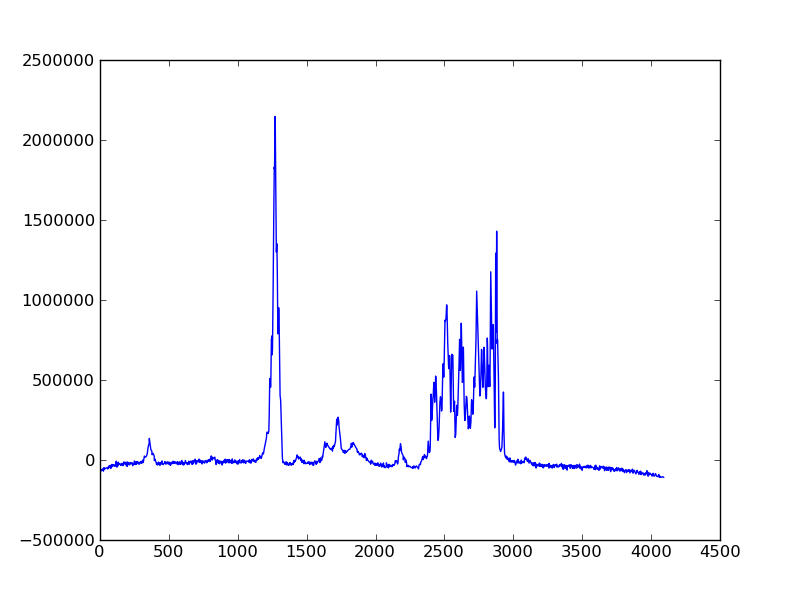
>>> import matplotlib.pyplot as plt
>>> dic, data = ng.pipe.read("test.ft")
>>> plt.plot(data)
[<matplotlib.lines.Line2D object at 0x8754fd0>]
>>> plt.savefig("plot_1d.png")
Here we have loaded the pyplot module from matplotlib (aliased as plt), and
used it to plot the 1D frequency domain data of a model protein. The resulting
figure is saved as plot_1d.png.
Alternately, the object-oriented interface from matplotlib can be used. This is especially useful when make more complicated plots. The above example would look something like this:
>>> import matplotlib.pyplot as plt
>>> dic, data = ng.pipe.read("test.ft")
>>> fig, ax = plt.subplots()
>>> ax.plot(data)
>>> fig.savefig("plot_1d.png")
A contour plot of 2D data can created in a similar manner:
>>> dic, data = ng.pipe.read("test.ft2")
>>> cl = [30000 * 1.2 ** x for x in range(20)]
>>> fig, ax = plt.subplots()
>>> ax.contour(data, cl)
<matplotlib.contour.ContourSet instance at 0x151e2f80>
>>> plt.show()
The plt.show() method raises an an interactive window for examining the plot:
matplotlib can be used to create more complicated figures with annotations, ppm axes and more. The Plotting Examples and Interactive Examples showcase some some of this functionality. For additional information see the matplotlib webpage
Additional resources
Detailed information about each module in nmrglue as well as the functions provided by that module can be found in the nmrglue Reference Guide or by using Python build in help system:
>>> help(ng.pipe.read)
A number of Examples using nmrglue to interact with NMR data are available. Finally documentation for the following packages might be useful to users of nmrglue:
Google Colabs and NMRglue
Here is the code that has been used in colabs …
import scipy
import numpy as np
!python -m pip install git+https://github.com/jjhelmus/nmrglue
Once the software has been installed, the tutorial is downloaded and
!wget https://storage.googleapis.com/google-code-archive-downloads/v2/code.google.com/nmrglue/tutorial_files.tar
unpacked
!tar -xvf tutorial_files.tar
putting us in a position to follow the tutorial.
For example,
import nmrglue as ng

dic,data = ng.pipe.read("test.fid")


print("The data has {0} dimensions and has shape {1} \nwhich are of type {2}."
.format(data.ndim, data.shape, data.dtype))
print("\nThe dictionary gives us the spectral width {0} \nand things like the name of the indirect dimension {1}".
  format(dic["FDF2SW"],dic["FDF1LABEL"]))
print("\nThe dictionary has {} keys which describe the spectral data.".format(len(dic.keys())))
and so on.