fitting example: fitting_t1_data
This example shows how to use nmrglue and the SciPy optimize module to fit T1 relaxation trajectories. Three scripts are used in the process.
The data used in this example is available for download.
First the extract_trajs.py script reads in box limits from boxes.in and
a list of spectra from spectra.in. The script integrates each peak in each
spectrum and writes the trajectory for each peak to disk as traj.npy in
NumPy .npy format.
#! /usr/bin/env python
# Scipt to extract trajectories from a series a 2D spectrum.

import nmrglue as ng
import numpy as np

# read in the integration limits and list of spectra
peak_list = np.recfromtxt("boxes.in")
spectra_list = np.recfromtxt("spectra.in")

# prepare the trajs records array
num_spec = spectra_list.size
num_peaks = peak_list.size
elist = [np.empty(num_spec, dtype="float") for i in xrange(num_peaks)]
trajs = np.rec.array(elist, names=list(peak_list.f0))

# loop over the spectra
for sn, spectra in enumerate(spectra_list):

    # read in the data from a NMRPipe file
    print "Extracting from:", spectra
    dic, data = ng.pipe.read(spectra)

    # loop over the integration limits
    for name, x0, y0, x1, y1 in peak_list:

        # integrate the region and save in trajs record array
        if x0 > x1:
            x0, x1 = x1, x0
        if y0 > y1:
            y0, y1 = y1, y0
        trajs[name][sn] = data[y0:y1 + 1, x0:x1 + 1].sum()

# normalize each trajectory
for peak in trajs.dtype.names:
    trajs[peak] = trajs[peak] / trajs[peak].max()

# save the trajectories records array to disk
np.save("traj.npy", trajs)
[boxes.in]
#Peak    X0     Y0      X0      Y1
A20     4068    938     4079    913
A24     3992    1013    4000    997
A26     4065    962     4075    940
A34     4009    985     4018    958
A48     4028    1034    4036    1010
C28     4035    1115    4044    1092
D36     3994    987     4003    973
D40     4076    802     4085    774
D46     4155    899     4163    883
D47     4053    967     4062    941
E15     4162    1022    4170    996
E19     4176    902     4185    875
E27     4036    1084    4044    1054
E42     4136    1055    4142    1026
E56     4107    821     4115    794
F30     4013    1060    4023    1031
F52     4097    828     4105    799
G09     4054    1249    4063    1220
G14     4068    1331    4077    1304
G38     4098    1254    4106    1227
G41     4091    1283    4099    1259
I06     4087    903     4096    884
data/Ytau_100.fid/test.ft2
data/Ytau_100000.fid/test.ft2
data/Ytau_250000.fid/test.ft2
data/Ytau_500000.fid/test.ft2
data/Ytau_750000.fid/test.ft2
data/Ytau_1000000.fid/test.ft2
data/Ytau_1500000.fid/test.ft2
data/Ytau_2000000.fid/test.ft2
data/Ytau_3000000.fid/test.ft2
data/Ytau_4000000.fid/test.ft2
The second script fit_exp_leastsq.py reads in this traj.npy file and the
T1 relaxation times associated with the spectra collected from time.dat.
Each trajectory is fit using the least squares approach. Other optimization
algorithms can be substituted with small changes to the code, see the
scipy.optimize
documentation). The resulting fits are saved to a fits.pickle file for
easy reading into python as well as the human readable fits.txt file.
#! /usr/bin/env python
# fit a collection to T1 trajectories to a decaying exponential

import scipy.optimize
import numpy as np
import pickle

# read in the trajectories and times
trajs = np.load("traj.npy")
t1 = np.recfromtxt("time.dat")

# fitting function and residual calculation
def fit_func(p, x):
    A, R2 = p
    # bound A between 0.98 and 1.02 (although fits do not reflect this)
    if A > 1.02:
        A = 1.02
    if A < 0.98:
        A = 0.98

    return A * np.exp(-1.0 * np.array(x) * R2 / 1.0e6)

def residuals(p, y, x):
    err = y - fit_func(p, x)
    return err

p0 = [1.0, 0.05] # initial guess

fits = {}
# loop over the peak trajectories
for peak in trajs.dtype.names:

    print "Fitting Peak:", peak

    # get the trajectory to fit
    traj = trajs[peak]

    # fit the trajectory using leastsq (fmin, etc can also be used)
    results = scipy.optimize.leastsq(residuals, p0, args=(traj, t1))
    fits[peak] = results

# pickle the fits
f = open("fits.pickle", 'w')
pickle.dump(fits, f)
f.close()

# output the fits nicely to file
f = open("fits.txt", 'w')
f.write("#Peak\tA\t\tR2\t\tier\n")
for k, v in fits.iteritems():
    f.write(k + "\t" + str(v[0][0]) + "\t" + str(v[0][1]) + "\t" + str(v[1]) +
            "\n")
f.close()
[time.dat]
# time in us
100
100000
250000
500000
750000
1000000
1500000
2000000
3000000
4000000
Results:
[fits.txt]
#Peak	A		R2		ier
E19	0.992583088163	0.165456904924	1
D36	0.978162369609	0.150387170038	1
E15	0.996022817946	0.0881391067001	1
G41	0.884746148818	0.528402076365	1
G09	0.993838313697	0.0974310406654	1
E56	0.978642097098	0.153694397368	1
D40	0.937320157503	0.32803199035	1
A34	1.00238376034	0.152055981221	1
E42	0.97955812576	0.201548076316	1
E27	0.957068222368	0.290667669811	1
F52	1.01437765462	0.063087299437	1
G38	1.00575140025	0.127826452523	1
C28	0.779226606115	0.680794315854	1
F30	0.955609064219	0.258560125202	1
G14	0.994898872827	0.108697405902	1
D47	0.993890875485	0.101193820532	1
D46	0.978622370865	0.074505374897	1
A48	0.984906624566	0.125792739083	1
A20	0.99998574293	0.102821608635	1
A24	0.923616582091	0.408644672104	1
A26	0.964157015536	0.252957335373	1
I06	0.997427797051	0.0604968616212	1
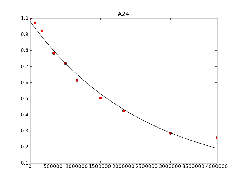
The last script pt.py reads in the fits, trajectories and T1
relaxation times and plots the experimental points and best fit to a series
of *_plot.png files.
[pt.py]
#! /usr/bin/env python
# Plot trajectories and fitting results

import pickle
import matplotlib.pyplot as plt
import numpy as np

# the same fit_func as in fit_exp_leastsq.py
def fit_func(p, x):

    A, R2 = p

    # bound A between 0.98 and 1.02 (although fits do not reflect this)
    if A > 1.02:
        A = 1.02
    if A < 0.98:
        A = 0.98

    return A * np.exp(-1.0 * np.array(x) * R2 / 1.0e6)

# read in the trajectories, fitting results, and times
fits = pickle.load(open("fits.pickle"))
trajs = np.load("traj.npy")
times = np.recfromtxt("time.dat")

sim_times = np.linspace(times[0], times[-1], 2000)

# loop over the peaks
for peak, params in fits.iteritems():

    print "Plotting:", peak
    exp_traj = trajs[peak]
    sim_traj = fit_func(params[0], sim_times)

    # create the figure
    fig = plt.figure()
    ax = fig.add_subplot(111)
    ax.plot(times, exp_traj, 'or')
    ax.plot(sim_times, sim_traj, '-k')
    ax.set_title(peak)

    # save the figure
    fig.savefig(peak + "_plot.png")
Results: