Relaxation trajectory analysis example
Introduction
This example is taken from Listing S12 - S15 in the 2013 JBNMR nmrglue paper. In this example a series of 3D NMRPipe files containing relaxation trajectories for a solid state NMR experment and analyzed.
Instructions
Execute python extract_traj.py to extract the relaxation trajectories from the data set. ‘XXX.dat’ files are created for the peaks defined in the boxes.in file. The spectra.in file defines which spectra the trajectories will be extracted from.
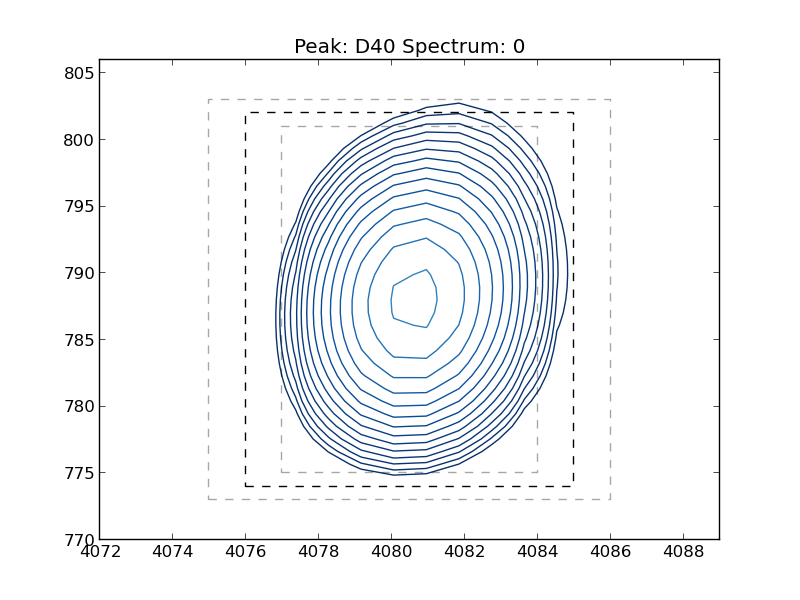
Execute python plot_boxes.py to create plots showing the peak and integration limits for all peaks defined in boxes.in. peak_XXX_spectrum_X.png files are created for all peaks and spectra. A example plot is provided as Figure 7 of the paper, which corresponds to peak_D40_spectrum_0.png
Execute python fit_exp.py to fit all relaxation trajectories. The fitting results are provided in the fits.txt file. The relaxation_times.in file defines the relaxation times for each spectra.
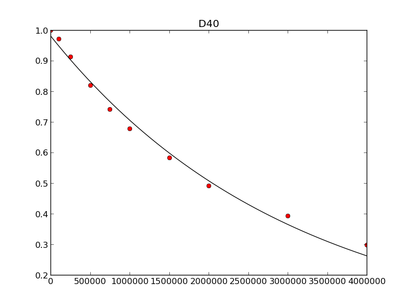
Execute python plot_trajectories to create plots of all experimental and fit relaxation tranjectories. This script creates a series of XXX_plot.png files. An example plot is provided as Figure 8 of the paper, which corresponds to D40_plot.png.
The data used in this example is available for download part1, part2, part3, part4.
Listing S12
import nmrglue as ng
import numpy as np

# read the integration limits and list of spectra
peak_list = np.recfromtxt("boxes.in", names=True)
spectra_list = np.recfromtxt("spectra.in")

# create an array to hold the trajectories
trajectories = np.empty((peak_list.size, spectra_list.size), dtype='float')

# loop over the spectra
for sn, spectra in enumerate(spectra_list):

    # read in the spectra data
    print "Extracting peak intensities from:", spectra
    dic, data = ng.pipe.read(spectra)

    # loop over the integration limits
    for i, (name, x0, y0, x1, y1) in enumerate(peak_list):

        if x0 > x1:
            x0, x1 = x1, x0
        if y0 > y1:
            y0, y1 = y1, y0

        # integrate the region and save in trajectories array
        trajectories[i][sn] = data[y0:y1 + 1, x0:x1 + 1].sum()

# write out the trajectories for each peak
for itraj, peak_traj in enumerate(trajectories):
    peak_traj /= peak_traj.max()    # normalize the peak's trajectory
    fname = peak_list.peak_label[itraj] + '.dat'
    f = open(fname, 'w')
    for v in peak_traj:
        f.write(str(v) + '\n')
    f.close()
Listing S13
import numpy as np
import nmrglue as ng
import matplotlib.pyplot as plt
import matplotlib.cm

# plot parameters
xpad = 5                        # padding around peak box on x-axis
ypad = 5                        # padding around peak box on y-axis
cmap = matplotlib.cm.Blues_r    # contour map (colors to use for contours)

# contour levels
cl = 30000 * 1.20 ** np.arange(20)

# read in the box limits and list of spectra
peak_list = np.recfromtxt("boxes.in", names=True)
spectra_list = np.recfromtxt("spectra.in")

# loop over the spectra
for spec_number, spectra in enumerate(spectra_list):

    # read in the spectral data
    dic, data = ng.pipe.read(spectra)

    # loop over the peaks
    for peak, x0, y0, x1, y1 in peak_list:

        if x0 > x1:
            x0, x1 = x1, x0
        if y0 > y1:
            y0, y1 = y1, y0

        # slice the data around the peak
        slice = data[y0 - ypad:y1 + 1 + ypad, x0 - xpad:x1 + 1 + xpad]

        # create the figure
        fig = plt.figure()
        ax = fig.add_subplot(111)

        # plot the contours
        print "Plotting:", peak, spec_number
        extent = (x0 - xpad + 1, x1 + xpad - 1, y0 - ypad + 1, y1 + ypad - 1)
        ax.contour(slice, cl, cmap=cmap, extent=extent)

        # draw a box around the peak
        ax.plot([x0, x1, x1, x0, x0], [y0, y0, y1, y1, y0], 'k--')

        # draw lighter boxes at +/- 1 point
        ax.plot([x0 - 1, x1 + 1, x1 + 1, x0 - 1, x0 - 1],
                [y0 - 1, y0 - 1, y1 + 1, y1 + 1, y0 - 1], 'k--', alpha=0.35)
        ax.plot([x0 + 1, x1 - 1, x1 - 1, x0 + 1, x0 + 1],
                [y0 + 1, y0 + 1, y1 - 1, y1 - 1, y0 + 1], 'k--', alpha=0.35)

        # set the title, save the figure
        ax.set_title('Peak: %s Spectrum: %i'%(peak, spec_number))
        fig.savefig('peak_%s_spectrum_%i'%(peak, spec_number))
        del(fig)
Listing S14
import glob

import numpy as np
from nmrglue.analysis.leastsqbound import leastsqbound

# exponential function to fit data to.
def fit_func(p, x):
    A, R2 = p
    return A * np.exp(-1.0 * np.array(x) * R2 / 1.0e6)

# residuals between fit and experimental data.
def residuals(p, y, x):
    err = y - fit_func(p, x)
    return err

# prepare fitting parameters
relaxation_times = np.loadtxt("relaxation_times.in")
x0 = [1.0, 0.10]  # initial fitting parameter
bounds = [(0.98, 1.02), (None, None)] # fitting constraints

# create an output file to record the fitting results
output = open('fits.txt', 'w')
output.write("#Peak\tA\t\tR2\t\tier\n")

# loop over the trajecory files
for filename in glob.glob('*.dat'):

    peak = filename[:3]
    print "Fitting Peak:", peak

    # fit the trajectory using contrainted least squares optimization
    trajectory = np.loadtxt(filename)
    x, ier = leastsqbound(residuals, x0, bounds=bounds,
                            args=(trajectory, relaxation_times))

    # write fitting results to output file
    output.write('%s\t%.6f\t%.6f\t%i\n' % (peak, x[0], x[1], ier))

output.close()  # close the output file
Listing S15
import numpy as np
import matplotlib.pyplot as plt

# exponential function used to fit the data
def fit_func(p,x):
    A, R2 = p
    return A * np.exp(-1.0 * np.array(x) * R2 / 1.0e6)

fitting_results = np.recfromtxt('fits.txt')
experimental_relaxation_times = np.loadtxt("relaxation_times.in")
simulated_relaxation_times = np.linspace(0,4000000,2000)

# loop over the fitting results
for peak, A, R2, ier in fitting_results:

    print "Plotting:", peak

    # load the experimental and simulated relaxation trajectories
    experimental_trajectory = np.loadtxt(peak + '.dat')
    simulated_trajectory = fit_func((A, R2), simulated_relaxation_times)

    # create the figure
    fig = plt.figure()
    ax = fig.add_subplot(111)
    ax.plot(experimental_relaxation_times, experimental_trajectory, 'or')
    ax.plot(simulated_relaxation_times, simulated_trajectory, '-k')
    ax.set_title(peak)
    fig.savefig(peak+"_plot.png")
Example input files
data/Ytau_100.fid/test.ft2
data/Ytau_100000.fid/test.ft2
data/Ytau_250000.fid/test.ft2
data/Ytau_500000.fid/test.ft2
data/Ytau_750000.fid/test.ft2
data/Ytau_1000000.fid/test.ft2
data/Ytau_1500000.fid/test.ft2
data/Ytau_2000000.fid/test.ft2
data/Ytau_3000000.fid/test.ft2
data/Ytau_4000000.fid/test.ft2
[boxes.in]
#peak_label    X0     Y0      X0      Y1
A20     4068    938     4079    913
A24     3992    1013    4000    997
A26     4065    962     4075    940
A34     4009    985     4018    958
A48     4028    1034    4036    1010
C28     4035    1115    4044    1092
D36     3994    987     4003    973
D40     4076    802     4085    774
D46     4155    899     4163    883
D47     4053    967     4062    941
E15     4162    1022    4170    996
E19     4176    902     4185    875
E27     4036    1084    4044    1054
E42     4136    1055    4142    1026
E56     4107    821     4115    794
F30     4013    1060    4023    1031
F52     4097    828     4105    799
G09     4054    1249    4063    1220
G14     4068    1331    4077    1304
G38     4098    1254    4106    1227
G41     4091    1283    4099    1259
I06     4087    903     4096    884
# time in us
100
100000
250000
500000
750000
1000000
1500000
2000000
3000000
4000000
Example output
[fits.txt]
#Peak	A		R2		ier
F30	0.981006	0.259152	1
D40	0.980906	0.328635	1
G14	0.994899	0.108697	1
A48	0.984907	0.125793	1
E15	0.996023	0.088139	1
D47	0.993891	0.101194	1
G38	1.005751	0.127826	1
F52	1.014378	0.063087	1
G09	0.993838	0.097431	1
A34	1.002384	0.152056	1
I06	0.997428	0.060497	1
E56	0.987760	0.157588	1
D36	0.985922	0.153331	1
A20	0.999985	0.102821	1
E27	0.993052	0.298782	1
D46	0.980000	0.074505	1
C28	0.980000	0.680741	1
E42	0.996588	0.210449	1
A26	0.989291	0.258348	1
E19	0.992583	0.165457	1
G41	0.980000	0.528399	1
A24	0.992186	0.417901	1